python, graphs, neo4j, dgraph, docker, webscraping
Unveiling Patterns in the Bundestag: A Graph‑Driven Exploration of Public Parliamentary Data
Morice NouvertneHow I transformed raw API responses into an interactive knowledge graph of parties, politicians, and committees—while testing both Neo4j and Dgraph along the way.
Why this project?
Germany’s Bundestag publishes an impressive amount of open data, but most of it lives in paginated JSON endpoints that are hard to grasp by eye. I was curious:
- Do certain parties dominate specific committees?
- Which MPs share the most topical interests or side jobs?
- Are there invisible “bridges” connecting otherwise distant party factions?
To answer those questions, I built a small pipeline that scrapes the freely accessible abgeordnetenwatch.de API, cleans and validates each record with Pydantic, and pours everything into a property graph database for exploratory queries and visualisation.
Responsible data use
Although all information is public‐domain, parliamentary data can still be politically sensitive. Throughout the project I followed three simple rules:
- Verbatim storage only – no enrichment with speculative attributes.
- No ranking or “scoreboard” rhetoric – patterns are shown, not judged.
- Reproducible code – every step can be verified against the original API.
From REST pages to a typed data layer
The API spans more than a dozen endpoints—parties, parliament periods, politicians, committees, side jobs, votes, and so on. To avoid schema drift I wrapped each endpoint in a dedicated Pydantic model. A shortened example for Party looks like this:
class Party(BaseModel):
id: int
entity_type: str
label: str
api_url: str
full_name: str | None = Field(alias="full_name")
short_name: str | None = Field(alias="short_name")
Each scraper inherits from a thin BaseScraper and pipes the raw JSON through its validator:
class PartyScraper(BaseScraper):
def fetch_all_parties(self, max_items=None, max_requests=None, pager_limit=1_000) -> list[Party]:
raw = self.fetch_all_data(max_items=max_items, pager_limit=pager_limit)
return [Party(**item) for item in raw]# invalid rows raise at source
The same pattern is repeated for ParliamentPeriod, Politician, Committee, Poll, Vote, Sidejob, … resulting in a set of clean, typed Python objects that are ready for graph import.
Why a graph database?
Parliamentary data is naturally relational:
- a Politician MEMBER_OF a Party
- holds multiple Mandates that PART_OF a ParliamentPeriod
- sits on several Committees that in turn discuss Topics
Instead of flattening those relations into SQL joins, I mapped them one‑to‑one into a property graph schema (excerpt below). That decision paid off when I started asking reachability questions such as “show me all MPs who have ever shared a committee and switched parties”.
Below is a snippet of the GraphQL style schema I used.
type Politician @node {
id: ID!
label: String!
party: Party @relationship(type: "MEMBER_OF", direction: OUT)
residence: City @relationship(type: "RESIDES_IN", direction: OUT)
...
}

type Committee @node {
id: ID!
label: String!
legislature: ParliamentPeriod @relationship(type: "PART_OF", direction: OUT)
}

type CommitteeMembership @node {
id: ID!
committee_role: String
committee: Committee @relationship(type: "HAS_MEMBER", direction: IN)
mandate: CandidacyMandate @relationship(type: "HAS_MEMBERSHIP", direction: IN)
}
Graph‑DB Comparison
| Neo4j 5 | Dgraph v23 | |
|---|---|---|
| Learning curve | Lower, great docs & Bloom UI | Steeper; GraphQL++ syntax takes practice |
| Import speed | neo4j-admin import finished 2 M nodes & 5 M rels in ~2 min | Bulk loader slightly faster but heavier RAM use |
| Ad‑hoc queries | Cypher felt more expressive for path patterns | DQL shines for graph traversals but lacks the wider ecosystem |
| Final choice | Kept Neo4j for its mature tooling and Cypher flexibility | Used only for early exploration |
Exploratory Findings
Please note that this party was selected at random and not based on any personal preference.
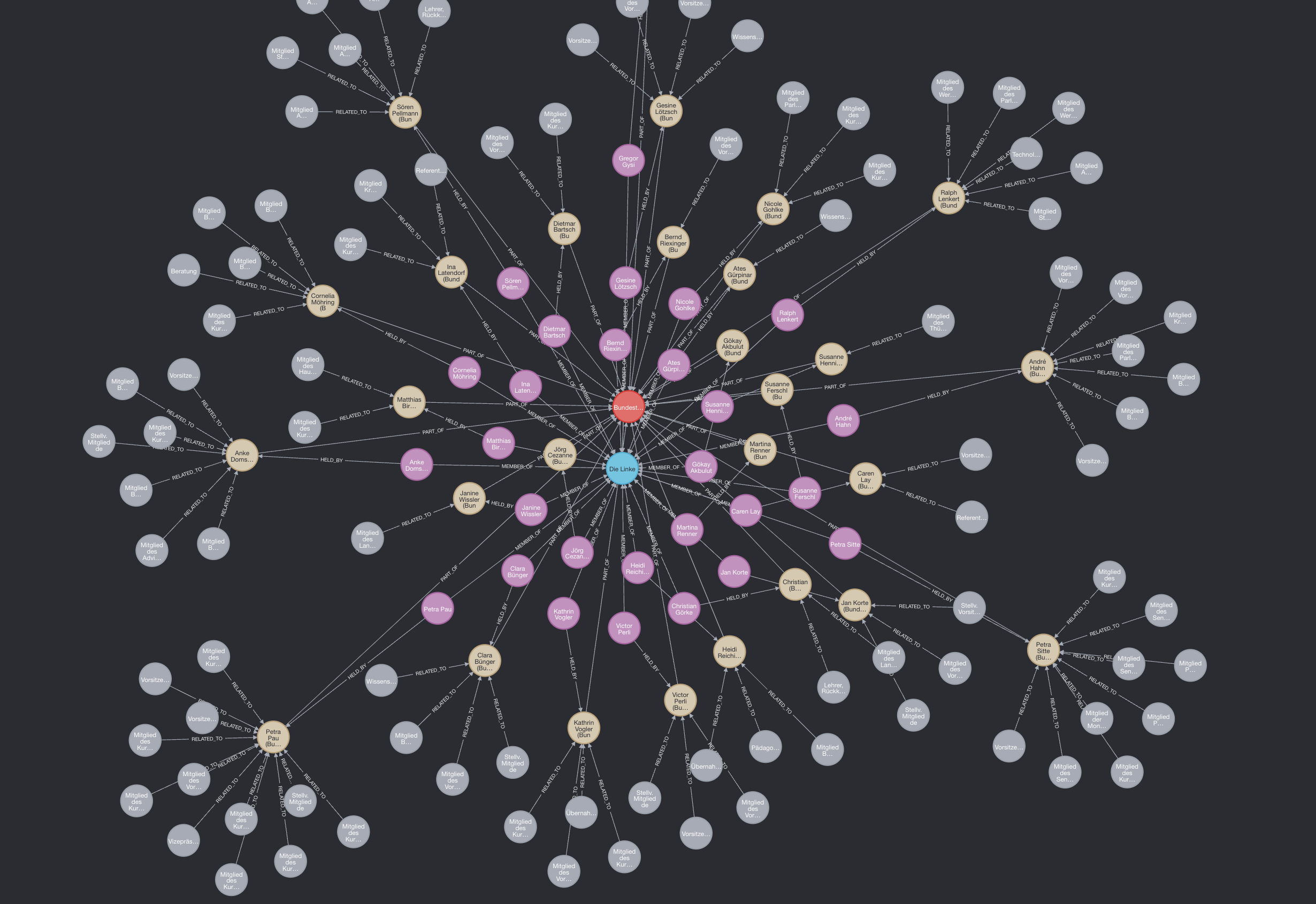 Network graph showing relationships between the German Bundestag, the political party Die Linke, and associated individuals, roles, and topics.
This graph explores the structural footprint of Die Linke within the Bundestag. At the center sits the Bundestag itself (red), flanked by Die Linke (blue) and a web of connected nodes:
- Purple and beige nodes represent individual politicians associated with Die Linke.
- Gray nodes reflect committees or positions held.
Edges are labeled with relationships such as:
- PART OF – linking individuals to the Bundestag or their respective committees,
- HELD BY – denoting positional roles,
- RELATED TO – associating people or groups with key policy areas.
This visualization offers an intuitive snapshot of how one political party’s human and thematic presence is distributed within federal parliamentary structures.
Note
An interesting way to explore this data is by mapping patterns in politicians’ educational backgrounds, part-time jobs, and organizational affiliations to uncover potential influences, conflicts of interest, or career trajectories within and across parties.
Tech stack in a nutshell
- Python 3.11 – scraping & ETL (async + httpx)
- Docker – Everything has been deployed using containers
- Pydantic v2 – data validation & type coercion
- Neo4j 5 – graph store, APOC for quick projections
- Jupyter – ad‑hoc Cypher notebooks and visual exports
What I learned
- Typed models save headaches – catching schema drifts early beats debugging malformed CSV imports later.
- Graphs expose hidden context – once relationships live as first‑class citizens, cross‑party collaboration patterns emerge without heavy SQL gymnastics.
- Tooling matters – both Neo4j and Dgraph are powerful, but a rich ecosystem (Bloom, APOC, community plugins) nudged me toward Neo4j for iterative exploration.
Potential next steps
- Temporal slicing – compare committee networks across legislative periods.
- Geo‑enrichment – link MPs’ constituencies to census data for regional context.
- Public mini‑dashboard – expose safe, aggregate‑only Cypher queries via a read‑only Neo4j instance.
All code, import scripts, and a reproducible Docker compose are available on GitHub (link forthcoming). If you have questions about the pipeline—or ideas for responsible, open analyses of parliamentary data—feel free to reach out!